1  What are we doing?

It is always good to start a course thinking about exactly what it is we are doing. Toward that end, we start with a question. What is the goal of doing (biological) experiments? There are many answers you may have for this. Some examples:

• To further knowledge.
• To test a hypothesis.
• To explore and observe.
• To demonstrate. E.g., to demonstrate feasibility.

More obnoxious answers are

• To graduate.
• Because your PI said so.
• To get data.

This question might be better addressed if we zoom out a bit and think about the scientific process as a whole. Below, we have a sketch of the scientific processes. This cycle repeats itself as we explore nature and learn more. In the boxes are milestones, and along the arrows in orange text are the tasks that get us to these milestones.

Figure 1.1: The cycle of science, adapted from Fig. 1.1 of P. Gregory, Bayesian Logical Data Analysis for the Physical Sciences, Cambridge University Press, 2005.

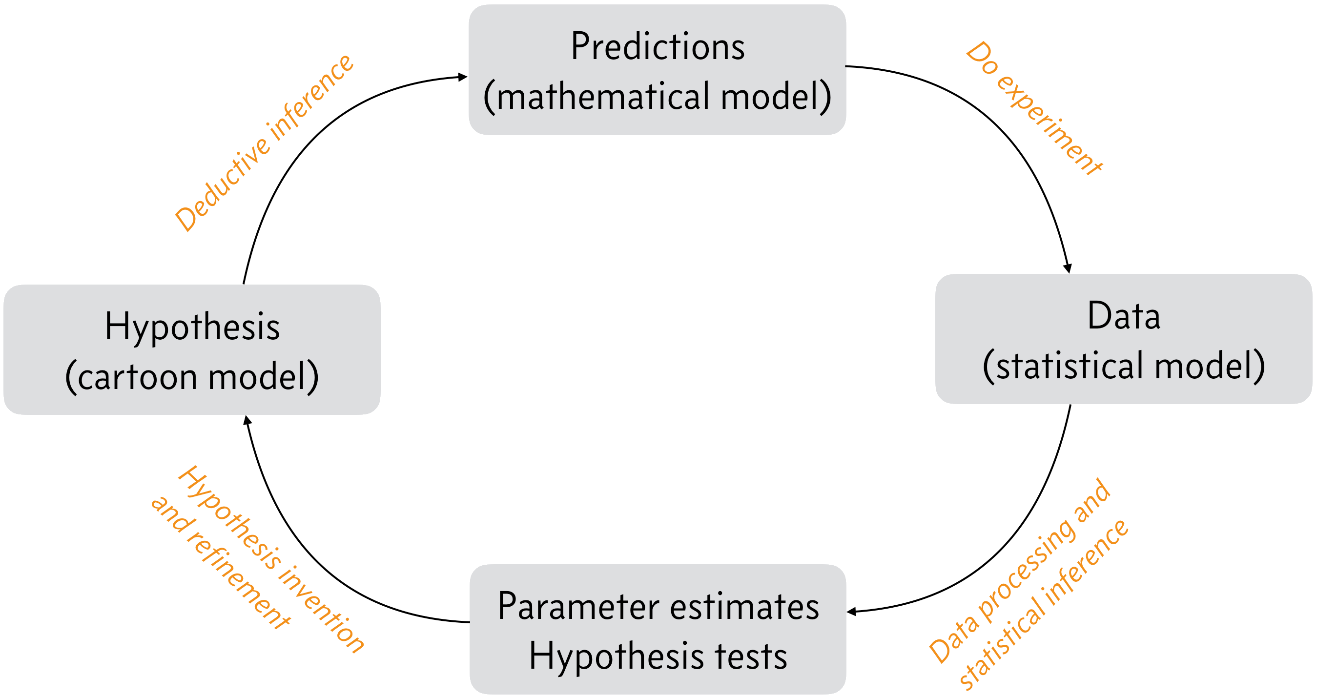
We start to the left with a hypothesis of how a biological system works, often expressed as a sketch, or cartoon, which is something we can have intuition about. Indeed, it is often a cartoon of how a system functions that we have in mind. From these cartoons, we can use deductive inference to move our model from a cartoon to a prediction. We then perform experiments to test our predictions, that is to assault our hypotheses, and the output of experiments is data. Once we have our data, we make inferences from them that enable us to update our hypothesis, thereby pushing human knowledge forward.

Let’s consider the tasks and their milestones in a little more depth. We start in the lower left.

• Hypothesis invention/refinement. In this stage of the scientific process, the researcher(s) think about nature, all that they have learned, including from their experiments, and formulate hypotheses or theories they can pursue with experiments. This step requires innovation, and sometimes genius (e.g., general relativity).

• Deductive inference. Given the hypothesis, the researchers deduce what must be true if the hypothesis is true. You have done a lot of this in your studies to this point, e.g., given X and Y, derive Z. Logically, this requires a series of strong syllogisms:

  • If A is true, then B is true.
  • A is true.
  • Therefore B is true.

  The result of deductive inference is a set of (preferably quantitative) predictions that can be tested experimentally.

• Do experiment. This requires work, and also its own kind of innovation. Specifically, you need to think carefully about how to construct your experiment to test the hypothesis. It also usually requires money. The result of doing experiments is data.

• Statistical (plausible) inference. This step is perhaps the least familiar to you, but this is the step that this course is mostly about. I will talk about what statistical inference is momentarily; it is too involved for this bullet point.

1.1 Data analysis pipelines

Let’s consider the lower right arrow in the figure above, going from a data set to updated hypotheses and parameter estimates, the heart of this course. We zoom in on that arrow, there are several steps, which we will call a data analysis pipeline, depicted below.

Figure 1.2: Data analysis pipeline. Each block represents a milestone along the pipeline and each arrow a task to bring you there.

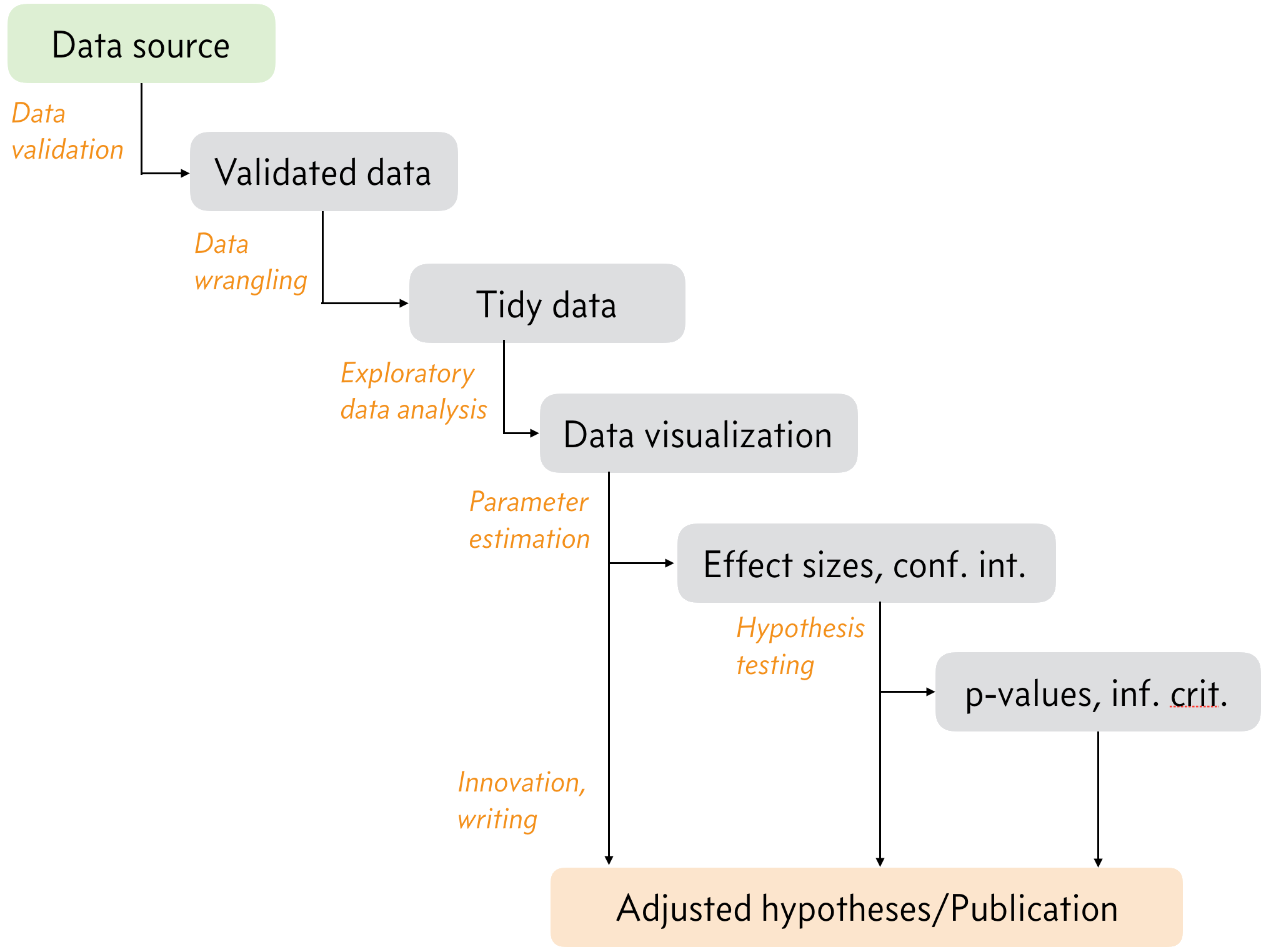
Let’s look at each step.

• Data validation. We always have assumptions about data coming from a data source into the pipeline. We have assumptions about file formats, data organization, etc. We also have assumptions about the data themselves. For example, fluorescence measurements must all be nonnegative. Before proceeding through the pipeline, we need to make sure the data comply with all of these assumptions, lest we have issues down the pipeline. This process is called data validation.
• Data wrangling. This is the process of converting the format of the validated data from the source to a format that is easier to work with. This could involved restructuring tabular data or extracting useful information out of images, etc. There are countless examples.
• Exploratory data analysis. Once data sets are tidy and easy to work with, we can start exploring them. Generally, this involves making informative graphics looking at the data set from different angles. Sometimes, this is sufficient to learn from the data, and we can proceed directly to updated hypotheses and publication, but we often also need to perform statistical inference, which is in the next two steps of the pipeline.
• Parameter estimation. This is the practice of quantifying the observed effects in the data, and in particular quantifying the uncertainty in our estimates of the effect sizes. This falls under the umbrella of statistical inference.
• Hypothesis testing. Also a technique of statistical inference, hypothesis testing involves evaluation of hypotheses about how the data were generated. This usually gives some quantitative measure about the hypotheses, but there are many issues with quantifying the “truth” of a hypothesis.

In this course, we will learn about all of these steps. We will spend roughly a third of the class on data validation and wrangling and exploratory data analysis, and the rest of the class on statistical inference.